On Ground Filtering

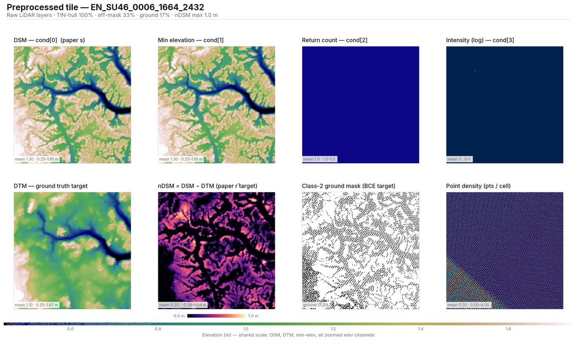
(This was not published on behalf of any company or organisation - only myself)

LiDAR and, in particular, the Environment Agency's dataset is the largest, publicly available dataset representing our country in three dimensions. Other countries' governments do this, but rarely on this scale, classified and freely available. This dataset provides the English national economy a boost and is used by many other national organisations, such as the Ordinance Survey, English Heritage, Forestry England and many government bodies to monitor the changing physical characteristics of England.

Since university, I have been focused on the problem of classifying this data into "ground" and "not ground". Whilst this seems a trivial question, it is very important for a range of specialities - flood mapping, archeology, digital twins, creating canopy models, and more. This is because knowing where the ground is is not only essential to working out the topography of the ground itself, but crucially, distinguishing and measuring what lies on-top of that ground.

In this project, I recreated the recently released paper GrounDiff which, through its original methodology, manages to overcome many of the hurdles that leave other leading approaches (KPConv, PTv3, PTD, SparseGF) stumbling on unseen terrain. Additionally, I released the code on Github for replication, with the results I achieved.

I would especially like to thank the authors of the paper, who recommended I adapt Palette, rather than working from scratch, and gave other helpful advice along the way. I'd also like to thank SE Gyges, an AI commentator, for giving advice about how to tune models best, when given a set of hyperparameters.

We can derive whether a point is a ground or not from its point cloud. Point clouds are generated from a LiDAR sensor, which in an aerial context is attached to a drone or a plane. The main advantage of LiDAR is that it can capture the height of the surfaces as well as gaps between vegetation or semi-occluded areas, which makes it useful for reaching spots that would be tricky for other sensors. 

The laser emitted is reflected from the surface below back into the sensor. The time this takes can allow for height to be derived. Along with the reflectance intensity, other metadata is stored for each point and recorded as part of the point cloud. For any given square metre of area, this process can be done a couple up to hundreds of times, depending on the sensor and the distance of the sensor to the ground.

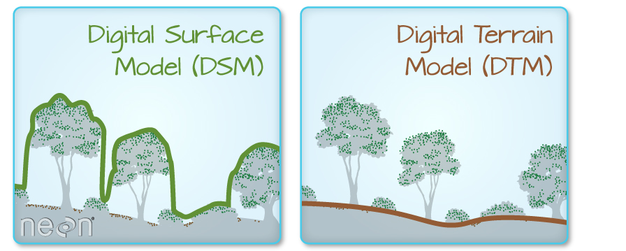
From these millions or even billions of points, we can derive a Digital Surface Model (DSM). The DSM is the surface collected from the aerial LiDAR, usually aggregated into a raster. For every unit of measurement, typically half a metre squared, the raster pixel represents the highest of the points of that unit. After this, it is necessary to interpolate missing gaps, using one of various algorithms.

The Digital Terrain Model (DTM) reflects the "bare-earth" ground surface, which, with the DSM, means we can measure the height of the objects above ground (the nDSM). This is done either through an algorithm that assumes that vegetation is mostly spiky, buildings are tall, water absorbs most LiDAR returns, and ground is mostly smooth - or one of various machine learning models. Then, manual refinement is done to ensure the ground points and other points (water, building, vegetation, roads etc.) are classified correctly.

To date, there have been many hundreds of papers to work out this DTM in an automated manner as accurately as possible. Through my research, I have read as many as possible. So far, I believe the best is GrounDiff. Some of its key advances includes:

• A diffusion model! We can treat the DSM as an image with noise, and the DTM as another image without noise. And then we can ask the model to work out how to remove the noise (buildings, vegetation) and figure out how best to get from one to another in unseen cases. ML models are very good at achieving this.
• nDSM (the height of an object above the relative ground, rather than its absolute height) is much easier to predict as a regression target, which can then be derived as a DTM. This is because estimating the relative position of something in potentially thousands of metres of space is a much greater challenge for most models, than a few dozen metres which is smaller and bounded.
• RMSE is the best metric to focus on. Previously models rely on IoU - which measures roughly how accurate the points are classified, factoring in false positives and false negatives. RMSE goes a step further and says it is more useful to penalise a building point (causing large RMSE errors) for most use cases than a point of grass (low RMSE error). This is because large RMSE errors make interpretation of the final result much more difficult, making it a truer representation of the usefulness of the underlying DTM.
• A gating mechanism. The model produces two outputs - the nDSM and the confidence that a point is ground or non ground. Where the confidence is high, the output can be directly modified. Where it is lower, the output is gated to a safer residual nDSM. This causes a significant increase in accuracy of the final output.
• The loss algorithm (the scoring system for the model) factors in both sharp surfaces, such as vegetation, as well as smooth surfaces, such as ground. How steep the difference between the output is compared to the true output is measured. Then, finally, the overall nDSM is matched against the true output to measure as a confidence score. Ablation testing showed this produced significantly better results than other cruder loss measures.
• PrioStitch allows us to run the model on a wider area at lower resolution, before running on individual tiles. This gives tiles additional context, addressing the 'global' vs 'local' problem addressed in other successful papers.

A change I made to this successful model was adding the minimum return as well as the maximum return, providing some extra context for vegetation and niche cases, giving the model more unique information.

This model was trained on the Environment Agency data. This data was stratified to 20 OS National Grid Squares, and split for training and validation. The model was trained for 28 hours on a RTX Pro 6000 Blackwell. For all other hyperparameters, which matched the original paper, the code has been uploaded to Github for public use.

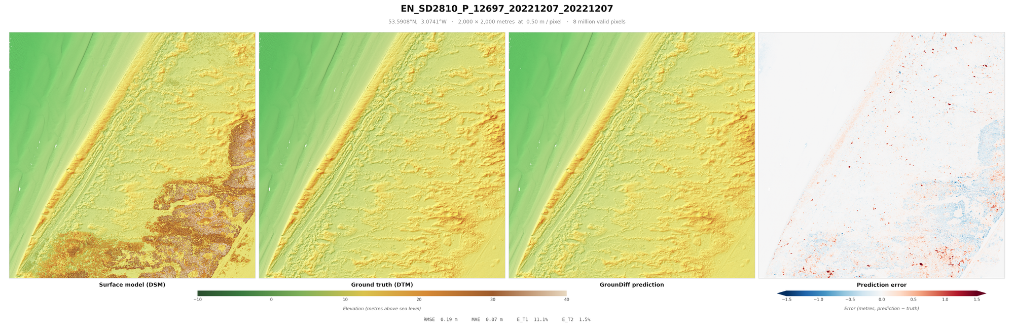
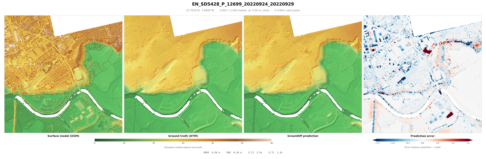
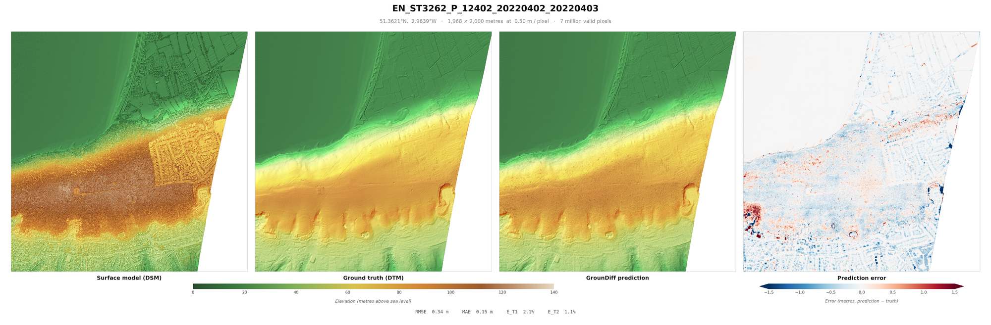
When looking at these results, it is worth factoring in some important caveats. One is sensor error (usually around 10cm RMSE), which measures the average error between the "true" location and the location measured on the z-axis. It is also worth considering the errors in classification that were made when making the English EA dataset - which would mean that no model can be a true representation of the DTM - “ground truth” is an exaggeration. Additionally, areas under buildings, vegetation etc. are included in the RMSE, inflating it from other papers (you might notice blue rectangles where buildings were in some of the below images). Some models do not even count this area at all in their metrics, but I included them to be be paper comparable. Further, these metrics are calculated on pixels, rather than points. Points can be derived by being 20cm from the DTM, to a relatively similar accuracy.

It is worth noting the images were generated using linear blend + Test Time Augmentation (TTA), as these are settings likely to be done in production to improve visual consistency. But overall results are achieved using a minimum blending and no TTA. The TTA and linear blending helps reduce RMSE by 5-10%, producing a more "conservative" product, but running TTA is more computationally and time consuming to get reliable figures on.

Were I do to do this again I would do ablations, testing TTA and whether adding the minimum points in pixels would help, as well as potentially intensity and return count. I would test different sizes, not only for the inputs, but stride and pixel resolution. The reason I didn't is testing is very expensive.

Overall Results

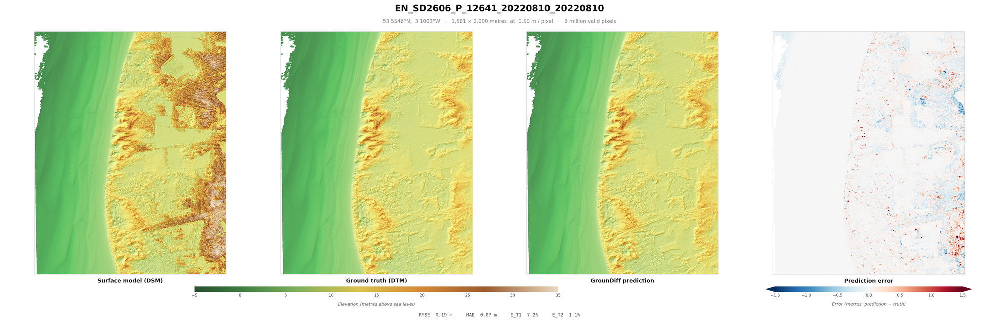
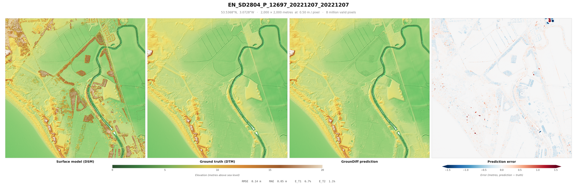
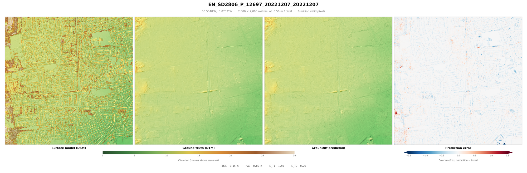
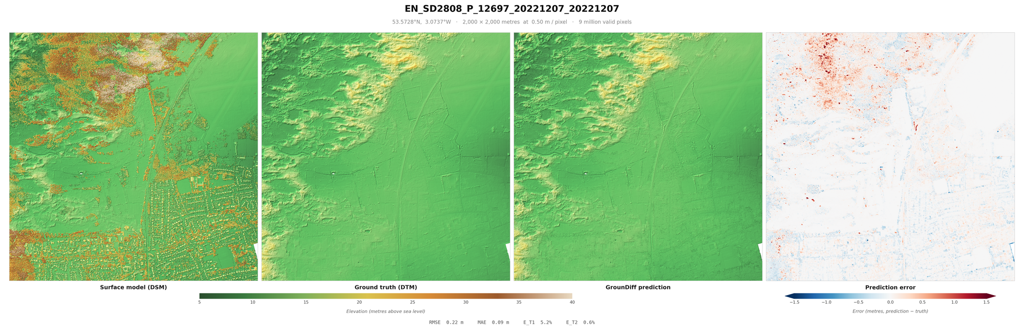
Result Images

I recommend loading these images full-screen, to get a sense of the terrain covered and objects removed.
These are a random sample of scenes with large drops (more likely to be difficult), as much of England is flat.

Training Metrics